
Aggregate supply
Aggregate supply
Aggregate supply (AS) is defined as the total amount of goods and services (real output) produced and supplied by an economy’s firms over a period of time. It includes the supply of a number of types of goods and services including private consumer goods, capital goods, public and merit goods and goods for overseas markets.
Components of AS
Consumer goods
Private consumer goods and services, such as motor vehicles, computers, clothes and entertainment, are supplied by the private sector, and consumed by households. For a developed economy, this is the single largest component of aggregate supply.
Capital goods
Capital goods, such as machinery, equipment, and plant, are supplied to other firms. These investment goods are significant in that their use adds to capacity, and increases the economy’s ability to supply private consumer goods in the future.
Public and merit goods
Goods and services produced by private firms for use by central or local government, such as education and healthcare, are also a significant component of aggregate supply. Many private firms such as those in construction, IT and pharmaceuticals, rely on contracts to supply to the public sector.
Traded goods
Goods and services for export, such as chemicals, entertainment, and financial services are also a key component of aggregate supply.
The Aggregate Supply curve
The simple law of supply suggests that firms will, in general, plan to produce more output at higher price levels.
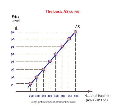
The basic AS curve
At higher price levels across the economy firms expect that they can sell their final products at higher prices, and there will be a positive relationship between the price level and aggregate supply.
Any increase in input prices (costs) which may follow is assumed to lag behind increases in the general price level. Because of this firms expect that they will benefit – at least in the short run – from a rise in the price level. Based on this we can derive a simple AS supply schedule, as shown below:
| PRICE LEVEL | AS £Bn |
| P8 | 650 |
| P7 | 600 |
| P6 | 550 |
| P5 | 500 |
| P4 | 450 |
| P3 | 400 |
| P2 | 350 |
| P1 | 300 |
| P | 250 |
The gradient of the AS curve
Different theories of the shape of the AS curve arise from different explanations about how real output responds to changes in aggregate demand. There are, essentially, three different views:
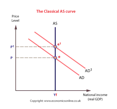
The Classical view
The Classical view of real output was that it was fixed at a particular level. At this level, all the factors of production in the economy would be fully employed. (Say at output 500).
| PRICE LEVEL | AS £Bn |
| P8 | 500 |
| P7 | 500 |
| P6 | 500 |
| P5 | 500 |
| P4 | 500 |
| P3 | 500 |
| P2 | 500 |
| P1 | 500 |
| P | 500 |
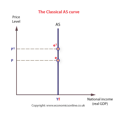
Changes in AD will only bring about changes in the price level, not the level of real output.
The Keynesian view
The Keynesian AS curve assumes that prices and wages are fixed until full employment is reached. Over the ‘Keynesian range’ there is spare capacity in the economy, the price level is stable, and real output can expand as a result of increases in AD without any inflationary pressure.
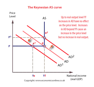
Beyond full employment, any changes in AD will bring about higher price levels. The Keynesian view of AS was adapted to show an ‘intermediate range’ where both unemployment and inflation could occur together.
| PRICE LEVEL | AS £Bn |
| P8 | 500 |
| P7 | 500 |
| P6 | 500 |
| P5 | 300 |
| P4 | 200 |
| P3 | 0 |
| P2 | 0 |
| P1 | 0 |
| P | 0 |

The adapted Keynesian AS curve is more realistic, and highlights the trade-offs that can occur between the price level and unemployment.
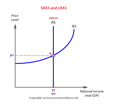
The ‘modern’ short run-long run view
To solve the problem of the Keynesian and Classical AS curve, modern economists tend to separate the short run AS curve (SRAS) from the long run AS (LRAS) curve. The short run is assumed to begin immediately after an increase in the price level (for example, as a result of an increase in AD), and ends when input prices (costs of production) have increased. Hence, during the short run producers are experiencing an increase in their ‘real’ prices and produce more output – and the supply curve slopes upwards.
Any increase in input prices (costs) which may follow is assumed to lag behind increases in the general price level. In this analysis, SRAS and LRAS are separated. This allows economists to be more flexible in their analysis of a modern economy. This can be seen in the following example:
| PRICE LEVEL | SRAS £bn | LRAS £bn |
| P8 | 650 | 500 |
| P7 | 600 | 500 |
| P6 | 550 | 500 |
| P5 | 500 | 500 |
| P4 | 450 | 500 |
| P3 | 400 | 500 |
| P2 | 350 | 500 |
| P1 | 300 | 500 |
| P | 250 | 500 |
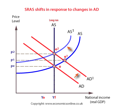
Shifts in the SRAS
The most likely cause of a shift in the SRAS curve is to accommodate changes in the short run AD curve.
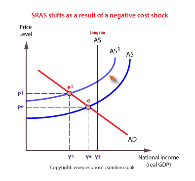
Other shifts in the SRAS curve are referred to a supply-side shocks, such as unexpected increases in oil prices or following crop failures, as illustrated below:
Shifts in the LRAS
The long run aggregate supply curve (LRAS) is the long run level of real output which is sustainable given the current quantity and quality of the economy’s scarce resources. Real output in the long run is not determined by the price level, and the long run AS curve will be vertical – short run changes in the price level do not alter an economy’s long-term output. This is equivalent to being on the edge of a country’s production possibility frontier.
The long run aggregate supply curve (LRAS) is shown as a vertical curve, at full employment. LRAS can shift if the economy’s productivity changes, either through an increase in the quantity of scarce resources, such as inward migration or organic population growth, or improvements in the quality of resources, such as through better education and training.
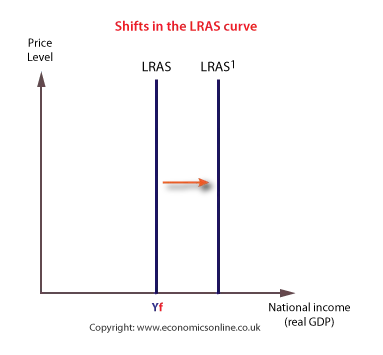
Shifts in LRAS are usually gradual and anticipated, unlike shifts in the SRAS which can be dramatic and unanticipated. LRAS can shift for many reasons, including:
- The level of spending on new technology, which enables an economy to produce in greater volume or improved quality – even using the same quantity of scarce resources.
- Long term inward investment from abroad, which enables increased production. Inward investment, like domestic investment, increases an economy’s productive capacity.
- Migration and population growth, which increases the quantity of human capital.
- Education and training, which increases the quality of human capital.
- Competition in product and labour markets, which improves efficiency and productivity.
- Effective supply-side policy, which creates the right environment for households to supply factors of production and for firms to produce output.
The effects of an increase in capital investment
The initial impact of investment is on the AD curve, which shifts to the right as investment (I) is a component of AD, show shown below:
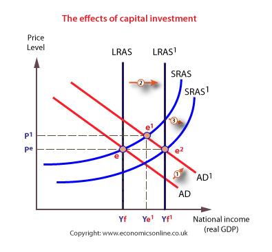
In the long run, the investment will increase the economy’s capacity to produce, which shifts the LRAS curve to the right. Finally, it is likely that production costs will fall as new technology increases efficiency and reduces average costs. This means that the SRAS curve shifts to the right. The combined effects are that the economy grows, both in terms of potential output and actual output, without inflationary pressure.
See more on investment