Isoquant Curves Simplified

What is an Isoquant Curve?

An isoquant curve is a curve that shows various combinations of two factors of production that a firm can use in order to get the same total output.

The term isoquant is derived from the Greek word ‘iso" which means equal, and ‘quant’ which means quantity. That is why the isoquant curve is also called an equal product curve or a production indifference curve.

Assumptions

The following assumptions are made while drawing the isoquant curves.

The time period is long run.
Technology remains constant.
A firm uses two factors of production, i.e., labour and capital.
Both factors of production are variable.
Both factors of production can be substituted.
Both factors of production are not perfect substitutes
All units of each factor of production are of equal quality.
The law of diminishing marginal returns is applicable for each factor of production.

The Building Blocks of Isoquants

To understand isoquants better, let's break down their essential components:

Inputs

The primary inputs considered in isoquant curves are capital and labour, although in real life, other factors of production may be included. Capital man-made resource such as machinery or other physical assets used in production while labour represents the number of workers or work hours.

Output

Isoquants revolve around a specific level of total output. This output is called total physical product (TPP). For instance, if we are studying an isoquant for producing 500 units of a product, all the input combinations on that isoquant will generate precisely 500 units of output.

Efficiency

Isoquants assume that firms aim to produce output efficiently. This means using the least amount of inputs possible to achieve a particular output level. Economists refer to this as the principle of technical efficiency.

Data Example

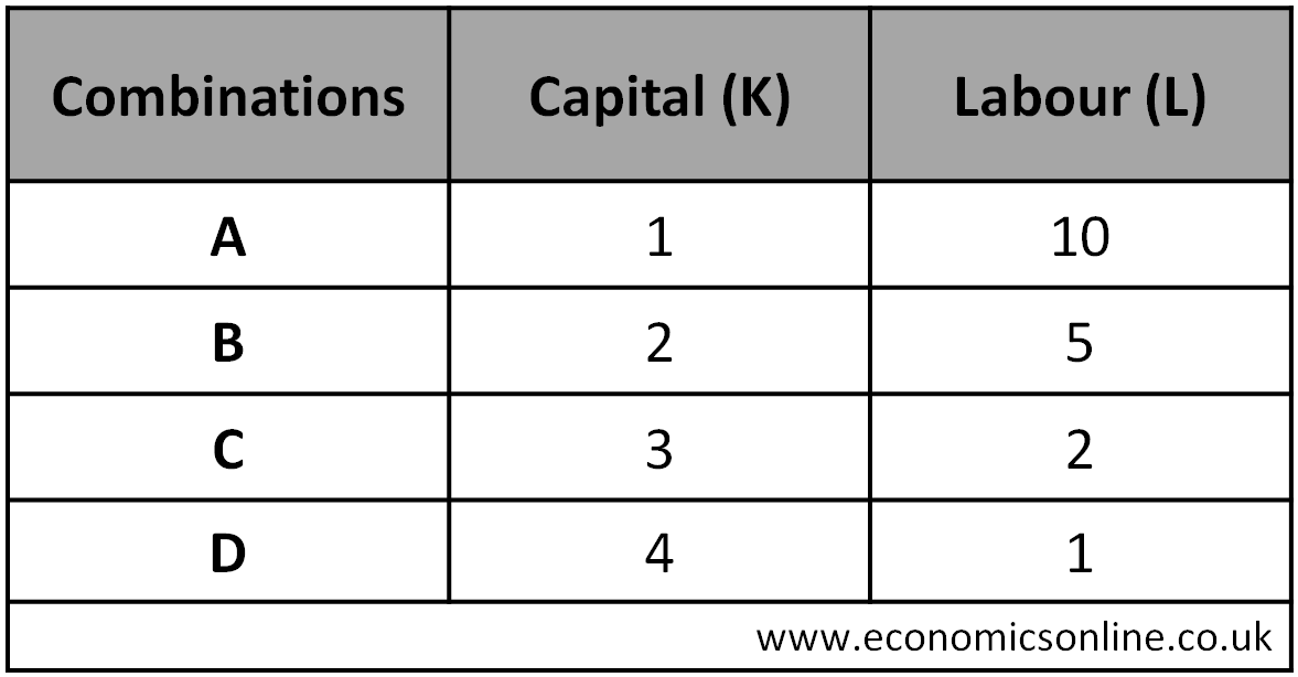
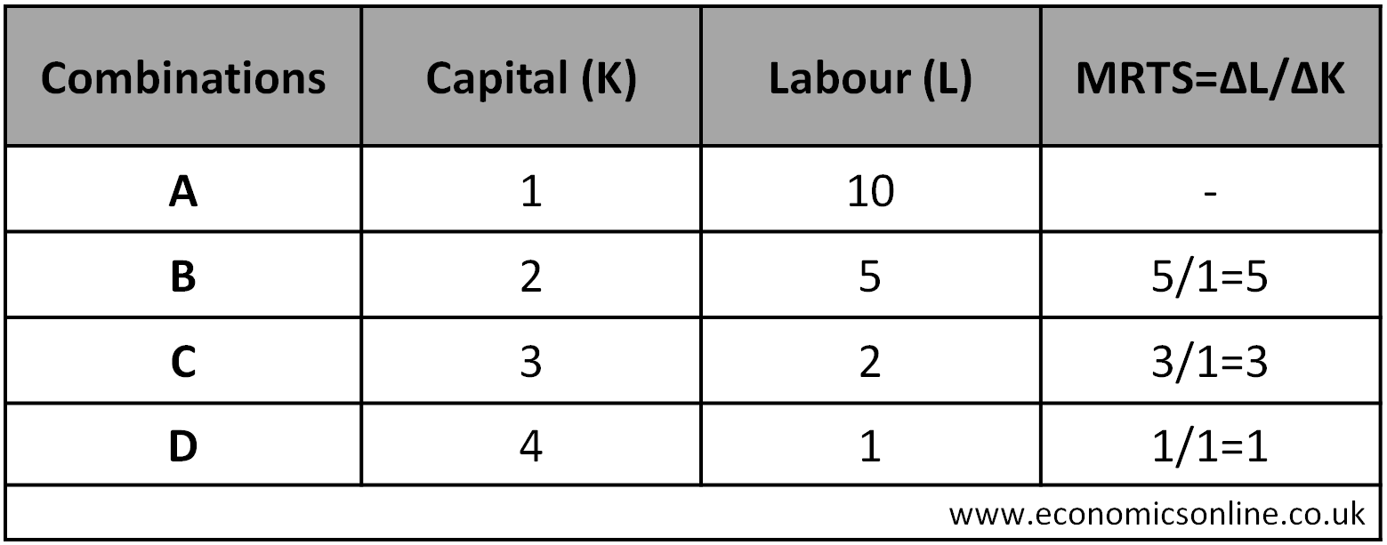
Let’s assume the following table which shows different combinations of capital (K) and labour (L) to produce the same total output or total physical product (TPP) of 500 units.

A table containing data values for constructing an isoquant curve.

Graph of an Isoquant

The following graph shows an isoquant curve for TPP of 500 units and is made by using data in the above table. On the horizontal axis (X-axis), we have taken the quantity of capital (K), while on the vertical axis (Y-axis), the quantity of labour (L) is taken. The graph of isoquant is a downward sloping curve which is convex to the origin.

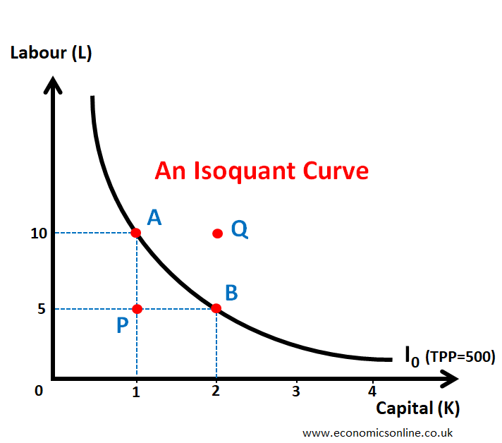
An isoquant curve shows possible combinations of two factors of production that a firm can use in order to get a given level of output. In the above example, this could be

1 unit of capital and 10 units of labour - Point A (labour intensive)

4 units of capital and 1 unit of labor - Point D (capital intensive)

Types of Points

Points on an Isoquant Curve

All points on the same isoquant curve are the combinations of labour (L) and capital (K), which give an equal quantity of total output (TPP = 500). For example, points A and B give the same total output of 500 units.

Points below an Isoquant Curve

All points below an isoquant curve give lower output. For example, point P will give an output lower than 500 units.

Points above an Isoquant Curve

All points above an isoquant curve give higher output. For example, point Q will give an output higher than 500 units.

Why is Isoquant Curve Downward Sloping?

An isoquant curve is downward sloping because in order to keep the total put constant, when capital is increased by one unit, labour must be decreased.

Why is an Isoquant Curve Convex to the origin?

An isoquant curve is convex to the origin or bowed inward because of the decreasing marginal rate of technical substitution (MRTS).

Marginal Rate of Technical Substitution (MRTS)

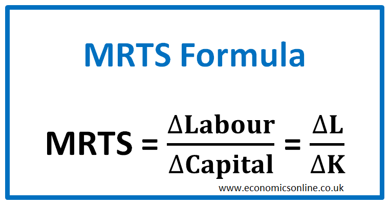
The marginal rate of technical substitution (MRTS) is the number of units of labour that must be sacrificed in order to increase capital by one unit to get the same total output. It is also called the marginal rate of factor substitution.

The MRTS formula is given below.

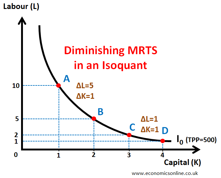
An image of the formula of MRTS (Marginal rate of technical substitution).

The diminishing MRTS is also shown in the following diagram.

A graph of isoquant curve illustrating diminishing marginal rate of technical substitution.

The calculations of the marginal rate of substitution (MRTS) are shown in the table below.

A table showing diminishing marginal rate of technical substitution.

Why is MRTS decreasing?

As we move along the same isoquant curve from one point to another, the total output remains constant. Hence, the output gained from using one more unit of capital must be equal to the output lost from using some units of labour.

MRTS is decreasing because of the law of diminishing marginal returns.

From Point A to Point B

MRTS = 5 (see above table), which means 5 units of labour must be sacrificed to increase capital by 1 unit in order to keep the output the same.

i.e. the output of 1 unit of capital is equal to the output of 5 units of capital

So capital is of higher value because of its lower quantity, and labour is less productive because of its higher quantity.

From Point C to Point D

MRTS = 1 (see above table), which means 1 unit of labour must be sacrificed to increase capital by 1 unit, in order to keep the output the same.

i.e. the output of 1 unit of capital is equal to the output of 1 unit of capital

So capital has become less productive with an increase in its quantity according to the law of diminishing marginal return, and labour is now more productive because of its reduced quantity.

The value or output of 1 unit of capital decreases with an increase in its quantity. So, the initial units of capital have a higher value (output) as compared to the later units. This is according to the law of diminishing marginal returns.

MRTS is the slope or gradient of an isoquant curve. This slope (MRTS) shows the rate at which labour and capital can be substituted.

Diminishing MRTS is the reason an isoquant curve is convex to the origin.

Characteristics of an Isoquant Curve

Slope

An isoquant curve is always downward-sloping.

Convexity

An isoquant curve is bowed inward or convex to the origin.

Not Touching the Axes

An isoquant curve cannot touch the X-axis or the Y-axis because a firm must use two factors of production as per the assumptions of an isoquant curve.

Non-Intersecting

Two isoquant curves cannot intersect because it violates the assumption of total output being the same for all points of the same isoquant.

Isoquant Maps

Firms have isoquant maps. A higher isoquant curve gives a higher total output.

Isoquant Map: Definition

A set or collection of Isoquant curves is called an isoquant map. It is shown by the following diagram:

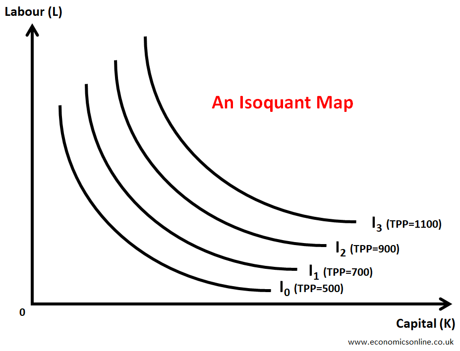
A higher isoquant curve will give a higher level of output, while a lower isoquant curve will give a lower output. A shift of an isoquant curve to a higher position indicates growth in the size of a firm. That will happen when a firm has more units of factors of production available for producing goods and services.

Practical Applications of Isoquants

Isoquants have several real-world applications:

Cost Minimisation

By analysing isoquants, firms can determine the most cost-effective combination of labour and capital to produce a specific level of output. This knowledge aids in minimising production costs, increasing profitability, and remaining competitive in the market.

Input Substitution

Isoquants help firms identify when and how to substitute one input for another while maintaining the same level of output. This is especially useful when facing changes in input prices or availability.

Resource Allocation

The isocost line is used with the isoquant map in order to find the optimal factor combination or an optimal combination of inputs.

This helps firms utilise scarce resources in the best possible way, i.e., to get maximum output at minimum cost. This will help firms optimise resource usage and improve economic efficiency.

Limitations of Isoquants

Isoquants are not easy to construct. The data may not be easily available.
Factors of production cannot be easily substituted.
Switching from labour intensity to capital intensity is difficult and involves other challenges like redundancies and labour issues.
Firms do not use only two factors of production.

Conclusion

An isoquant curve is the locus of possible combinations of factors of production that can produce the same output. The Isoquant curve may appear as complex graphs, but they are quite easy to understand. Understanding isoquants can enable firms to make better decisions about input combinations and resource allocation.