Indifference curves

Introduction

The origins of indifference analysis can be traced back to the work of late 19th Century Irish economist Francis Edgeworth, and later, to Italian economist Vilfredo Pareto.

The starting point for indifference analysis is to identify possible baskets of goods and services which yield the same utility (usefulness, or satisfaction) to consumers.

It is assumed that individuals, faced with a budget constraint, will choose the basket that maximises their total utility – in other words, they will act rationally when allocating their budget. The search to identify bundles of goods and services that yielded the same utility marked a significant point in the development of consumer theory as indifference analysis does not require the direct measurement of utility for a single good. Indifference analysis, therefore, provided a solution to the long-standing problem of how to measure utility.

Cardinal and ordinal utility

In indifference analysis, it is not necessary to establish an objective and observable measure of utility (referred to as cardinal utility), but simply to identify those baskets of goods and services that consumers are indifferent to, and are equally preferred. Indifference analysis only requires that we rank consumer’s relative preferences and, thereby, establish an order of preference, referred to as ordinal utility.

Assumptions underlying indifference analysis

Indifference curve analysis makes four essential assumptions about consumer choices and decision-making.

Completeness

This assumption states that there are only two propositions we can make about a consumer’s choices between bundles of goods – that they prefer one bundle to another, or they are indifferent to them. No other options are possible.

Transitivity

This principle rules out illogical decision-making, and states simply that if bundle A is preferred to B, and B is preferred to C, then it must be true that bundle A is preferred to C.

Consistency

Indifference curve theory assumes that preferences will be consistent, given the same information and constraints. In other words, if the decision-making context for an individual remains constant on both Monday and Tuesday, then a consumer will have the same order of preference on Tuesday as on Monday.

Preference for more

Finally, indifference analysis, as with all tradtional mico-economic perspectives, assumes that consumer’s prefer more of a ‘good’ than less of it. This also means that consumers would prefer less of a ‘bad’ than more of it.

Constructing an indifference curve

A single indifference schedule can be constructed to show all those possible combinations of goods that would yield the same utility to the consumer.

For example, consider the following schedule which shows a hypothetical consumer’s indifference to a range of combinations of just two items of clothing – woollen sweaters (x) and cotton socks (y). Each combination yields the same level of utility.

Reveal figures for indifference

From this we can derive an indifference curve for these bundles.

Indifference curve

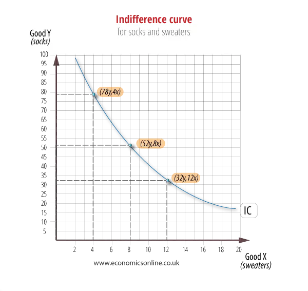
The consumer is indifferent to any combination on the indifference curve – baskets of 78y and 4x, 52y and 8x, and 32y and 12x are equally preferred.

The Diminishing Marginal Rate of Substitution

The shape of an indifference curve reflects a consumer’s willingness to substitute one good for another, which is measured as the ‘marginal rate of substitution’ (MRS).

The MRS indicates how much of good y a consumer is prepared to give up to get one more unit of x (and, as such, is the inverse of marginal utility).

Formally, the MRS is:

The MRS diminishes the further along the curve we move, hence the slope of an indifference curve is convex to the origin. An indifference curve cannot have a flat gradient as this would run counter to the principle of the diminishing marginal rate of substitution.

Apples and oranges

Assume an individual likes both apples and oranges and these are the only goods they purchase, and that, at the moment, they have a basket which contains 10 apples and only 1 orange. In order to gain an additional orange (from 1 to 2), the consumer must sacrifice apples, which currently form the majority of the basket. Given the imbalanced basket, and the relative shortage of oranges in that basket and the relative abundance of apples, it is like that the consumer would give up several apples to gain the extra orange – say, 4 apples for 1 more orange – in which case, the MRS is 4.

However, with one more orange in the basket, the consumer would now offer fewer than before to gain an extra orange (from 2 to 3) – let us assume 2 apples – the MRS falls to 2.

Apples and oranges example

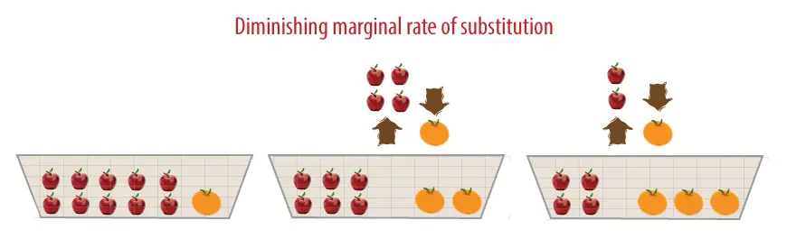
As the basket slowly switches from being an apple-rich basket to a more balanced basket, the consumer is less likely to give up so many apples for yet another orange. Hence, the marginal rate of substitution diminishes with each marginal orange that is added to the basket. The diminishing rate of substitution reflects the diminishing marginal utility of more oranges.

Sweaters and socks

In terms of the sweaters/socks example above, we can see the falling MRS as more sweaters (good x) are added to the basket – the MRS falls continuously the more x we have. Having 1 sweater and increasing this to 2 means being prepared to lose 13 pairs of socks, while increasing sweaters from 8 to 9 means sacrificing only 5 pairs of socks. Moving from 15 to 16 sweaters means sacrificing only 2 pairs of socks.

Diminishing MRS

Indifference curve maps

Indifference curve analysis suggests that the rational consumer has many such points of indifference, depending on the budget available to them, and on other significant factors which affect the consumer’s preferences between two goods.

For example, in the diagram below there are four indifference curves, each one representing a different set of indifference points relating to different levels of utility.

Indifference curve map

Indifference curves do not cross

It is inconsistent to suggest than an indifference curve would cross another one – this is logically impossible.

Indifference curves cannot cross

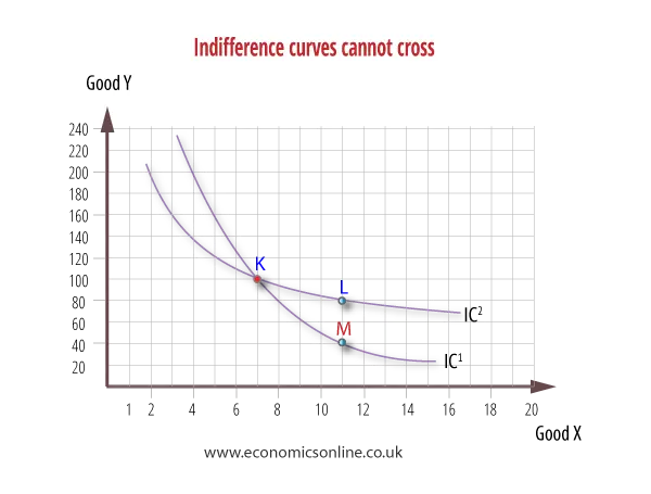
Given that all points on an indifference curve have identical utility, in the above diagram K equals M on IC¹, but also equals L on IC²! However, this is impossible, assuming the consumer is rational, as it would mean that L also equals M. This would not be rational as baskets L and M contain identical units of x (11) but different units of y, with L having 80, and M having 40. A rational consumer would prefer L to M! Hence, indifference curves cannot cross.

Budgets and budget lines

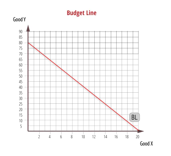
The budget line for a consumer shows all possible combinations of goods that can be bought at a specific income level (budget) and with specific prices of goods.

If we take our previous example of sweaters (good x) and socks (good y) and assuming the price of x is 20, and y is 5, with income at 400, then the following combinations are all possible.

Figures for budget line