
Aggregate demand
Aggregate demand
Economists use a variety of models to explain how national income is determined, including the aggregate demand – aggregate supply (AD – AS) model. This model is derived from the basic circular flow concept, which is used to explain how income flows between households and firms.
Aggregate demand (AD)
Aggregate demand (AD) is the total demand by domestic and foreign households and firms for an economy’s scarce resources, less the demand by domestic households and firms for resources from abroad.
Aggregate demand consists of the amount households plan to spend on goods (C), plus planned spending on capital investment, (I) + government spending, (G) + exports (X) minus imports (M) from abroad. The standard equation is:
AD = C + I + G + (X – M)
Aggregate demand and the circular flow
Aggregate demand can be illustrated by reference to the circular flow of income.
Aggregate demand is generated as income is transferred to spending as a result of the circular flow of income. Income is spent on consumer goods and services (C) plus spending on capital goods by firms (I). Spending is also generated by government when it allocates resources to public goods, merit goods and income transfers, such as pension benefits. Finally, there is ‘net overseas spending’, which is overseas spending on an economy’s exports of goods and services, less what the economy spends on importing goods and services.

Prices and output
The AD – AS model provides a framework to show how the level of AD and AS respond to changes in the price level and in turn, how changes aggregate demand and supply affect an economy’s national output (income) and its price level.
Example of aggregate demand
AD can be found by adding-up the value of all the individual components at various average price levels.
| PRICE LEVEL | C | I | G | X | M | AD |
| 200 | 300 | 50 | 100 | 50 | 450 | |
| 180 | 320 | 60 | 105 | 100 | 425 | |
| 160 | 340 | 70 | 110 | 150 | 400 | |
| 140 | 360 | 80 | 115 | 200 | 375 | |
| 120 | 380 | 90 | 120 | 250 | 350 | |
| 100 | 400 | 100 | 125 | 300 | 325 | |
| 80 | 420 | 110 | 130 | 350 | 300 | |
| 60 | 440 | 120 | 135 | 400 | 275 |
Exercise – calculate AD.
AD and the price level:
Apart from imports, the components of AD are inversely related to prices. Each component responds differently to changes in prices, in other words they have different elasticities with respect to the price level.
For example, we can assume that overseas demand is elastic with respect to price, because overseas consumers can choose from many global suppliers. This makes them highly sensitive to changes in the prices of imported products.
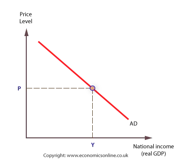
The aggregate demand curve
The AD curve shows the relationship between AD and the price level. It is assumed that the AD curve will slope down from left to right. This is because all the components of AD, except imports, are inversely related to the price level.
For convenience, the AD curve is normally drawn as a straight line, though it can be argued that it is more likely to be non-linear, many suggesting it has a rectangular hyperbola shape.
It is also claimed that the downward slope of the AD curve reflects ‘normal’ macro-economic conditions, and that in a deep recession, the AD curve could become vertical.
Trade, liquidity and wealth effects
The AD curve slopes down because the components of AD are inversely related to the price level. Price changes have a number of important affects on aggregate behaviour of households and firms.
There are three main effects to consider.
The price level and international trade – the ‘trade’ effect
The first effect, on overseas trade, is perhaps the most obvious one. A rise in domestic prices makes exports less competitive and imports more competitive; hence exports (X) are likely to fall and imports (M) are likely to rise. Both of these reactions combine to create a trade effect, with lower aggregate demand at the higher price level.
The price level and liquidity – the ‘liquidity/interest rate’ effect
When the price level increases, households and firms need to spend more money to continue to consume the scarce resources they need. This makes them relatively ‘short of cash’ than they were at the lower price level. The liquidity of an asset refers to how easily it is converted to cash, with cash itself being ‘perfectly liquid’. The loss of liquidity associated with a rise in the price level forces some households and firms to borrow from banks, which reduces the liquidity of banks. In response, banks are likely to raise interest rates as compensation for this lost liquidity. The banks need to keep a certain amount of their reserves in a highly liquid form to meet any unexpected increase in demand for cash.
As a result of the lost liquidity, interest rates are forced to rise, and both household and corporate spending may fall. Hence, aggregate demand is lower at the higher price level.
The price level and the value of wealth – the ‘wealth’ effect
Given that interest rates will rise as financial markets readjust to the higher price level, there are likely to be further ‘knock on’ effects on household (and corporate) wealth. Higher rates may lead to a fall in house prices, or at least slow-down house price inflation, and create a negative wealth effect. The same may be true for those households and firms that rely on income from shares. Rising interest rates tend to reduce corporate profits and reduce share values – again creating a negative wealth effect. A lower price level will, of course, have the reverse effect, that is to create a positive wealth effect on AD. The combined effect of these wealth effects is to alter consumer and corporate spending, and hence alter the level of AD.
When combined, the above effects explain why aggregate demand responds inversely to changes in the price level.
These effects should not be confused with other exogenous affects, which will shift the whole position of the AD curve.