Image showing factory doing production
Constant Returns to Scale
Constant returns to scale refer to the phenomenon whereby the output of a production process increases in proportion to the inputs, regardless of the scale of the operation. In other words, if the inputs to a production process are doubled, the output will also double, regardless of the size of the operation.
Here the word ‘scale’ means the amount of all the factors of production (FOP) held by a firm including units of labor, land and capital. If the scale is doubled, it means all the factors of production are doubled. Firms can increase the scale only in the long run. Firms can increase the scale only in the long run. In the long run all the inputs are variables.
One way to understand constant returns to scale is to consider the long run production function, which describes the relationship between inputs and output in a production process and can be explained with the help of the law of returns to scale.
The Law of Returns to Scale
If all the factors of production are increased with the same proportion i.e. the scale is increased in long run, then increase in the level of outputs can be of the following types.
1. Increasing Returns to Scale
2. Constant Returns to Scale
3. Decreasing Returns to Scale
Increasing Returns to Scale
If an increase in all the factors of production by the same proportion (an increase in the scale) leads to more than proportionate increase in the output, then the change in the output is called increasing returns to scale. This means that the output is increased by a greater proportion than the increase in total input. It means the rate of change of output is more than the rate of change of inputs. This is the first category (variation) of returns to scale.
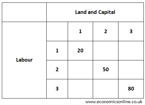
In above table, increasing returns to scale (IRS) are shown.
When all the FOP are increased from 1 to 2 then
% increase in FOP = [(2–1)/1] X 100% = 100% and
% increase in output Q (Shown on diagonal of table) = [(50–20)/20] X 100% = 150%.
When all the FOP are increased from 2 to 3 then
% increase in FOP = [(3–2)/2] X 100% = 50% and
% increase in output Q (Shown on diagonal of table) = [(80–50)/50] X 100% = 60%.
Again % increase in output is greater than % increase in the scale. Hence this is called increasing returns to scale.
Constant Returns to Scale
If an increase in all the factors of production by the same proportion (an increase in the scale) leads to the same proportionate increase in the output, then the change in the output is called constant returns to scale. It means the rate of change of output is equal to the rate of change of inputs. This is the second category(variation) of returns to scale.
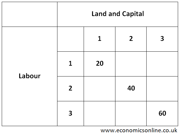
In above table, constant returns to scale (CRS) are shown.
When all the FOP are increased from 1 to 2 then
% increase in FOP = [(2–1)/1] X 100% = 100% and
% increase in the output Q (Shown on diagonal of table) = [(40–20)/20] X 100% = 100%
When all the FOP are increased from 2 to 3 then
% increase in FOP = [(3–2)/2] X 100% = 50% and
% increase in the output Q (Shown on diagonal of table)= [(60–40)/40] X 100% = 50%
Again % increase the output is equal to % increase in the scale. Hence this is constant returns to scale.
Decreasing Returns to Scale
If an increase in all the factors of production by the same proportion (an increase in the scale) leads to less than proportionate increase in the output, then the change in the output is called decreasing returns of scale. It means the rate of change of output is less tha the rate of change of inputs. This is the third category(variation) of returns to scale.

In above table, decreasing returns to scale (DRS) are shown.
When all the FOP are increased from 1 to 2 then
% increase in FOP = [(2–1)/1] X 100% = 100% and
% increase in the output Q (Shown on diagonal of table) = [(30–20)/20] X 100% = 50%
When all the FOP are increased from 2 to 3 then
% increase in FOP = [(3–2)/2] X 100% = 50% and
% increase in the output Q (Shown on diagonal of table) = [(36–30)/30] X 100% = 20%
So % increase in the output is less than % increase in the scale. Hence this is decreasing returns to scale.
Factors affecting the Returns to Scale
The level of technology and the efficiency of the production process can affect the returns to scale. If a company is able to adopt new technologies or improve the efficiency of its production process, it may experience increasing returns to scale, where the output increases at a faster rate as the inputs are increased. On the other hand, if a company is using out-dated technologies or has an inefficient production process, it may experience decreasing returns to scale, where the output increases at a slower rate as the inputs are increased.
The level of specialisation and division of labour within the organisation can affect the returns to scale. If a company is able to specialise and divide tasks among workers, it may be able to achieve increasing returns to scale, as the increased specialisation can lead to increased efficiency and productivity. On the other hand, if a company lacks specialisation and division of labour, it may experience decreasing returns to scale, as the lack of specialisation can lead to reduced efficiency and productivity.
Returns to Scale and the Long Run Average Cost (LRAC)
One important aspect of constant returns to scale is its impact on the cost structure of a business. The diagram below shows long run average cost (LRAC). The quantity is taken on the X-axis and cost is taken on the Y-axis.
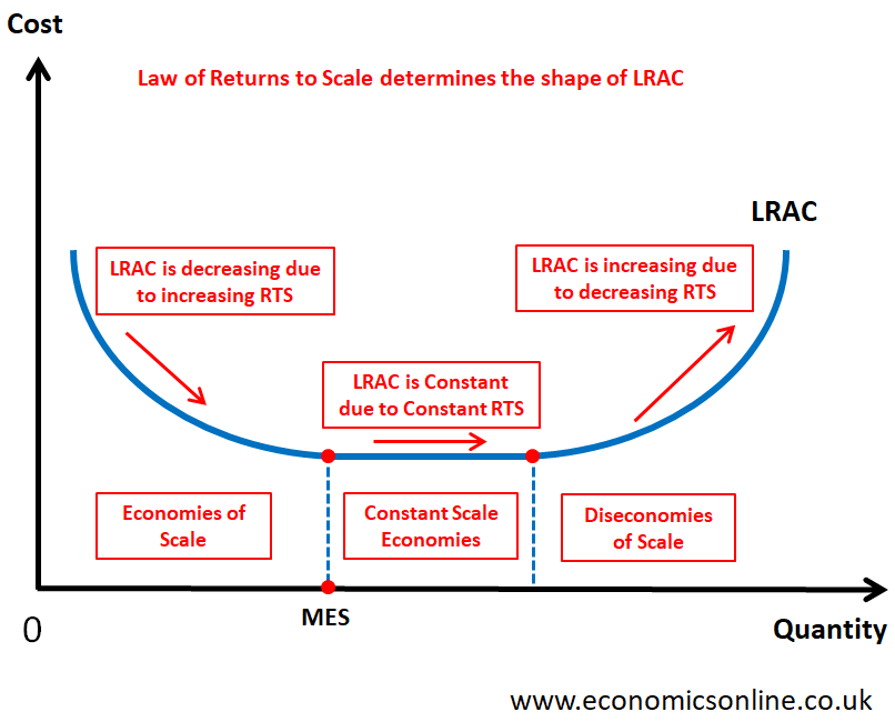
A production process with constant returns to scale exhibits a constant LRAC curve, meaning that the average cost of production remains the same as the scale of production increases. This is shown by the horizontal (straight line portion) of LRAC curve in the diagram and is called the constant scale economies.
This is in contrast to a production process with increasing returns to scale, which exhibits a downward-sloping LRAC curve (economies of scale), and a production process with decreasing returns to scale, which exhibits an upward-sloping long run AC curve (diseconomies of scale).
In the diagram, the lowest output for which LRAC is minimum is called the Minimum Efficient Scale (MES).
This should be kept in mind that returns to scale and diminishing marginal product of labour (MPL) are different concepts where the former works in the long run and the latter works in the short run.
Understanding the returns to scale of a production process is important for businesses as it can help to identify the most efficient production methods and allocate resources in the most cost-effective manner.