
A close-up photo of a person holding a leather wallet with money.
Marginal Propensity to Save (MPS)
Introduction
The marginal propensity to save (MPS) measures the strength of the relationship between changes in savings and changes in household disposable income. In economics, MPS is useful in determining the impact of changes in savings on the economy as a whole. In this article, we will discuss the definition of MPS, its calculation and its significance in economic analysis.
MPS Definition
The marginal propensity to save (MPS) is the change in household savings due to a change in household disposable income. It is the additional amount of money which consumers save out of their additional income. MPS is a reflection of the willingness to save for each additional dollar of income of individuals.
MPS Formula
MPS is calculated by dividing the change in saving by the change in in household disposable income. The MPS formula is given below:
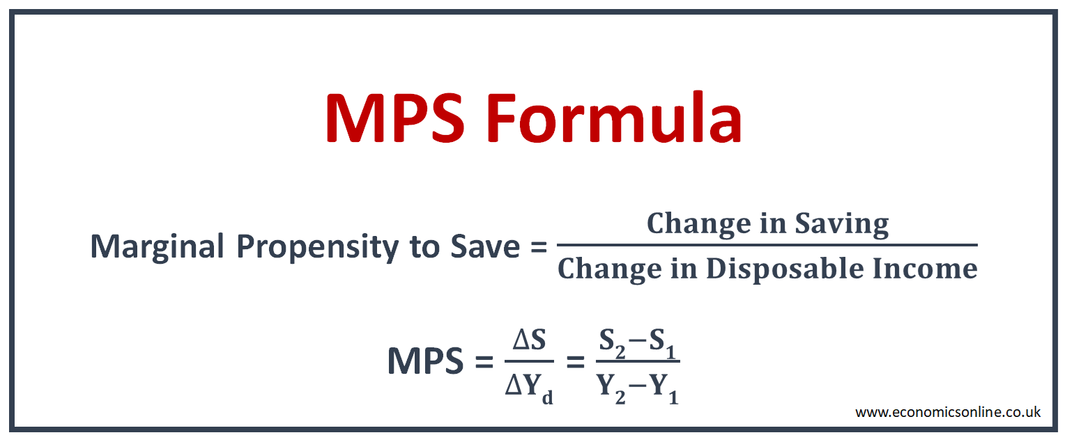
Marginal Propensity to Save = Change in Saving / Change in Disposable Income
MPC = ΔS / ΔYd
Where ΔS is the change in saving and ΔYd is the change in disposable income.
Some key points about the marginal propensity to save are:
- The marginal propensity to save always varies between 0 and 1.
- The value of the marginal propensity to save is 1 if the whole income is saved.
- The value of the marginal propensity to save is 0 if the whole income is consumed. This means that the increase in income has no effect on saving.
- MPS of 0.5 means that $0.50 is saved out of every extra $1 income.
MPS Example
Suppose that the household disposable income is increased from $100 to $200 and the savings are increased from $60 to $120. Here, the change in income is $100, while the saving changes are $60.
ΔYd = $100
ΔS = $60
MPS = ΔS / ΔYd = $60 / $100 = 0.6
The marginal propensity to save is 0.6, which is between 0 and 1. MPS of 0.6 means that out of every extra $1 income, $0.60 is saved.
MPS is the slope or gradient of S-Function. In Keynesian economic theory, economists and analysts use the value of MPS to understand the relationship between income and saving. It is also used to understand the activities of the household sector in the whole economy.
MPS value is not always the same. Seasonal trends affect the value of the marginal propensity to save for every individual. As individuals spend more money on purchases during the holiday season, their marginal propensity to save is low. After these seasons, individuals prefer to save more, resulting in a high value of MPS.
MPS and the Saving Function
The saving function, also known as the Keynesian saving function, is a theoretical relationship between saving and household disposable income. The equation of the saving function is typically represented as S = S0 + MPS (Yd), where S is saving, Yd is disposable income, S0 is autonomous saving (dissaving or negative saving that occurs independently of income), and MPS is the marginal propensity to save. The MPS represents the slope of the saving line and shows the extent to which an increase in disposable income leads to an increase in saving. It is illustrated in the following diagram.
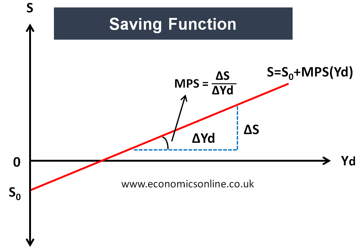
In the above graph, disposable income (Yd) is taken on the horizontal x-axis, while saving is taken on the vertical y-axis. MPS is the slope or gradient of the saving function.
MPS and the Shape of Saving Function
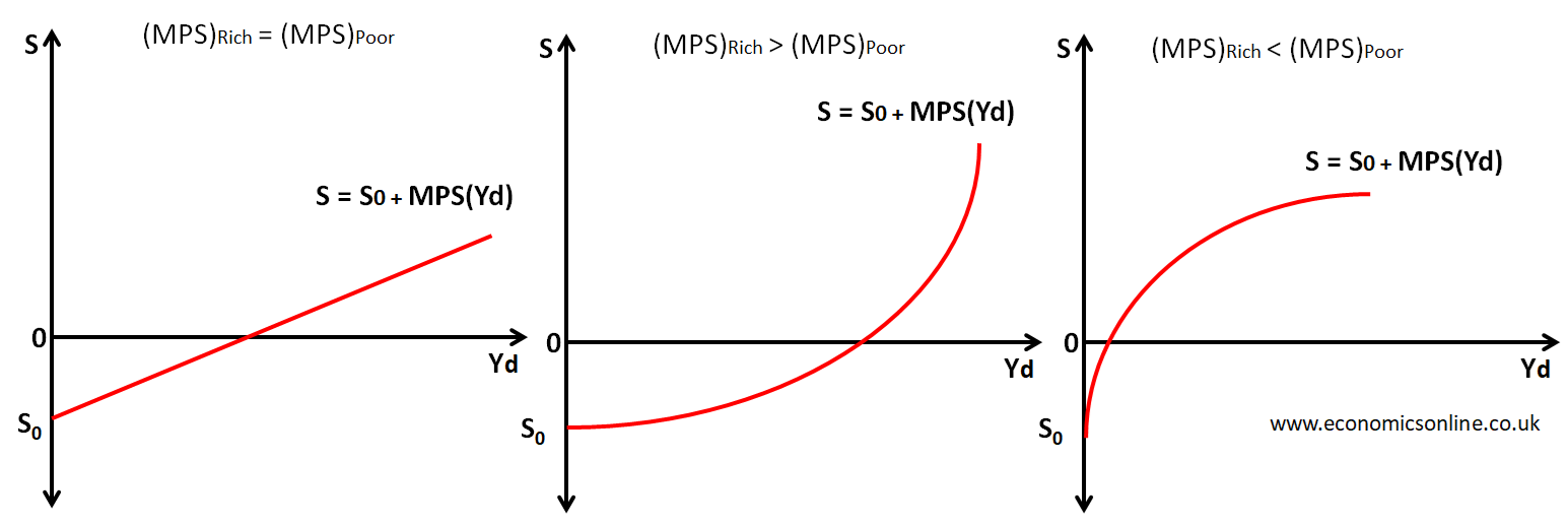
MPS determines the shape of saving function.
1. MPS is constant for a straight line saving function: (MPS)Rich = (MPS)Poor
2. MPS is increasing for an increasing sloped saving function: (MPS)Rich < (MPS)Poor
3. MPS is decreasing for a decreasing sloped saving function: (MPS)Rich > (MPS)Poor
This is illustrated by the following graphs:
Generally, a high level of household income indicates a higher marginal propensity to save. When people become rich, they have enough money to fulfil their needs, and a higher portion of the extra income goes to savings instead of being spent on general needs. But high income can also change people’s consumption patterns, as they may shift their patterns towards luxury goods to showcase exclusivity, such as a lavish lifestyle, high-end vehicles, and expensive holidays.
Significance of MPS
MPS is an important concept in macroeconomics because it helps in understanding the relationship between saving and disposable income. MPS also helps in understanding the behaviour of the household sector in the economy along with the calculation of the multiplier.
MPS and MPC
The marginal propensity to consume (MPC) is the additional consumption due to an additional income. The relationship between MPC and MPS depends on the type of economy, and is explained below:
In two-sector closed economy, where there is a household sector and a firm sector, MPS = 1 – MPC
In a three sector closed economy, where there are household sector, firm sector and government sector, MPS = 1 – MPC – MRT. Here, MRT is the marginal rate of tax.
In four sector open economy, where there are household sector, firm sector, government sector and foreign sector, MPS = 1 – MPC – MRT – MPM. Here, MPM is the marginal propensity to import.
MPS and the Circular Flow of Income
In the circular flow of national income, saving is a leakage or a withdrawal because it is the money which is put aside for future use and is taken out of the circular flow. A high value of MPS means that more money is saved out of the additional income, which leads to an increase in withdrawals from the circular flow of national income.
MPS and the Multiplier Effect
The multiplier effect is the tendency of a small change in injections or withdrawals to bring about a large change in national income. The size of the Keynesian multiplier depends on the value of MPS.
In two sector economy, the multiplier (K) = 1 / MPS.
In three sector economy, the multiplier (K) = 1 / (MPS+MRT).
In four sector economy, the multiplier (K) = 1 / (MPS+MRT+MPM).
The strength of the multiplier depends on the value of MPS. The higher the MPS, the weaker the multiplier effect, and vice versa. If the MPS is 0.2 in two sector economy, for example, then the value of the multiplier effect is 1 / 0.2 = 5, meaning that a change in injections of $100 would result in a final increase in national income of $500. If the MPS is 0.4, then the multiplier effect is 1 /0.4 = 2.5.
Factors Affecting the Marginal Propensity to Save
The following are some factors that influence the marginal propensity to save:
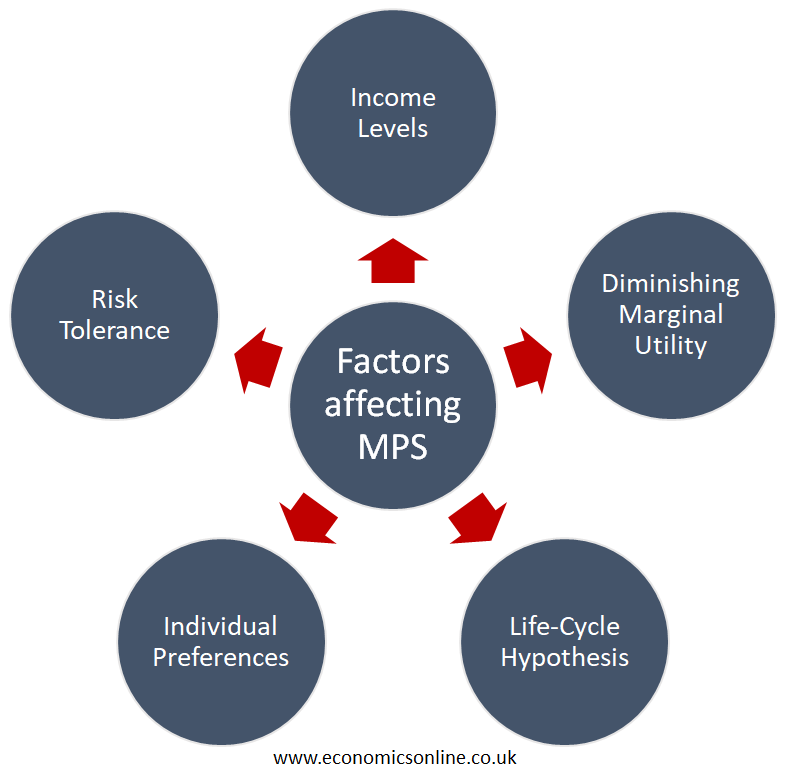
Income Levels
Income levels affect the value of consumers’ MPS. When people have a low income level, they prefer to spend a high portion of income to buy necessities to fulfill their needs and save a smaller portion of their income. At low level of income, individuals have a low value of MPS. With a higher income, an individual consumer saves more, resulting in a high value of MPS. The value of MPS is different for the rich and the poor. A high MPS value is one of the reasons why the rich get richer.
Diminishing Marginal Utility
When people have more income, they can buy more quantities of the goods, leading to a diminishing marginal utility from their use or consumption. This leads to a fall in MPC and an increase in MPS. This is one of the factors due to which the rich have a higher value of MPS.
Life-Cycle Hypothesis
The theories of life cycle related to individual spending assume that individuals wish to smooth out their consumption patterns with the passage of time. In an individual’s life cycle, when he is in the studying phase, his marginal propensity to save may be zero, as students have less money which may be just enough to fulfill daily needs. When he gets a better-paid job, now he is in a position to increase his saving amount. But when he reaches mid-working life, most of his income goes to saving, and his MPS is high, because of putting money aside for retirement.
Individual Preferences
All individuals have their own preferences; many do not follow the same life-cycle hypothesis, and fail to save. Some individuals are more rigid about current-income bias. These individuals prefer to fulfill today's consumption needs instead of saving for the future.
Risk Tolerance
Those individuals who are risk-averse are willing to save more for their future and minimise their consumption leading to a high value of MPS. But those individuals who are risk-loving do not save much for their future. They spend money freely on their current needs leading to a low value of MPS.
Conclusion
In conclusion, marginal propensity to save is an economic measure of the tendency of people to save money out their additional disposable income. MPS is an important metric in economic theory and is used in various concepts such as Keynesian theory of income and employment determination and the multiplier.