Labour markets

Labour markets

The demand for labour – marginal productivity theory

The demand for factors of production is derived from the demand for the products these factors help make.  For example, if mobile phones are in greater demand, then the demand for workers in the mobile phone industry will increase, ceteris paribus.

Demand and the wage rate

The demand for labour will vary inversely with the wage rate. To understand this we need to consider the law of diminishing returns. This states that if a firm employs more of a variable factor, such as labour, assuming one factor remains fixed, the additional return to extra workers will begin to diminish. To explore this process, we need to consider the total physical product (output) produced by a series of workers, which will enable us to measure the individual output from each additional worker – the marginal physical product (MPP).

Consider the following data for a small firm producing handmade.

Workers	Total Physical Product	Marginal Physical Product
1	1000
2	1900	900
3	2700	800
4	3400	700
5	4000	600
6	4500	500
7	4900	400

If we know the price of each candle, we can then calculate the value of the marginal physical product produced by each worker. For example, if candles are £2 each, the firm can calculate the revenue derived from each worker’s physical output. The value of the extra output is called marginal revenue product (MRP) and this is calculated by multiplying MPP and price, as follows:

Workers	Total Physical Product	Marginal Physical Product	Marginal Revenue product
1	1000
2	1900	900	1800
3	2700	800	1600
4	3400	700	1400
5	4000	600	1200
6	4500	500	1000
7	4900	400	800

Deriving a demand curve

We can now find the number of workers that would be employed by a profit maximising firm at various wage rates. The profit maximising firm will employ workers up the point where the marginal benefit, in terms of the MRP, equals the marginal cost of labour (MCL), which in this case is the wage rate (W).

For example, at a wage rate of £1,200, the firm will employ 5 workers, because at 5 workers, MRP = MCL. At a lower wage of £800, the firm will employ 7 workers, and so on.  This means that a demand curve can be derived. In labour market theory, the demand for labour is identified as MRP=D.

The supply curve of labour in a competitive market

In a perfectly competitive labour market, where the wage rate is determined in the industry, rather than by the individual firm, each firm is a wage taker and the actual equilibrium wage will be set by in the market, as follows:

The simple model of market wage

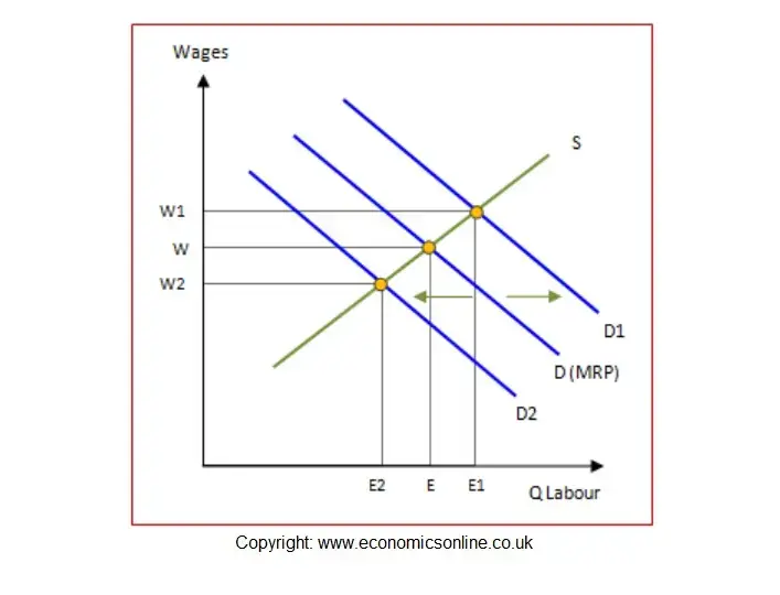
The competitive market wage rate, and the quantity of labour employed, is determined by the interaction of demand and supply. The equilibrium wage rate is the rate that equates demand and supply, as illustrated below.

Equilibrium wage rate

Labour supply for the whole market is assumed to be positively related to the wage rate, and the market supply curve slopes upwards.

Changes in market wage

Market wage may change following a change in an underlying condition of demand or supply.

Demand can change, and the demand curve will shift, under a number of circumstances, including changes in:

• The productivity of labour.
• The price of the product.
• Demand for the product.

Shifts in the demand for labour

Labour supply can change under a number of circumstances, including changes in:

• The length of the working week.
• Participation rates.
• Demographic factors, such as migration, and changes in the age structure of the population.
• The qualifications and skills needed.
• The length of training.

Shifts in the supply curve

Monopsonists

The special case of the monopsonist – the single buyer of labour – is an important one.  A monopsonist is a single buyer of labour, such as De Beers, the diamond producer, and the major employer of diamond workers in South Africa. Monopsonists are common in some small towns, where only one large firm provides the majority of employment.

Because the monopsonist is the only employer in the industry, it must raise the marginal wage to attract new workers into the industry if it wishes to employ more labour. The supply curve of labour is not the same as the marginal costs of labour because, as the only employer, the monopsonist must pay all existing workers the same rate as the new workers. Hence, when attracting new workers, the marginal cost of labour is greater than the existing average cost of labour.

This can be illustrated with the example of a hair salon in a small town.

Workers (Hair dressers)	Wage to attract new workers (W) = Average Cost of Labour, per hour	Total cost of labour (TCL) (assuming all workers paid the new wage rate)	Marginal expenditure = Marginal cost of labour (MCL), per hour	Marginal Revenue Product (MRP),  per hour
1	10	10		70
2	20	20 + 20 = 40	30	60
3	30	30 + 30 + 30 = 90	50	50
4	40	160	70	40
5	50	250	90	30
6	60	360	110	20
7	70	490	130	10

The monopsonist’s marginal cost of labour and supply curve

Assuming the monopsonist tries to maximise profits, it will demand labour up to the point where MCL = MRP. This will occur at 3 hairdressers, where the MCL and MRP are both £50 per hour, as shown below:

However, the wage paid to the workers is only £30. In this case, the monopsonists is said to be exploiting the workers by paying less than the MRP – i.e. wages are £30 per hour, and the MRP is £50 per hour, meaning that the monopsonist has gained £20. It can achieve this because it does not have to pay the full value of the MRP.

However, if there are several hair salons in the town, each salon will have to bid up the wage rate in order to attract sufficient hairdressers so that they can maximise their individual profits. The competitive wage rate would exist where the wage to attract workers (the labour supply curve) equals the MRP curve, at a rate of £40, and employing 4 hairdressers.

What is a union fixes a minimum wage?

A union minimum wage

A union can represent workers and seek to increase the benefits to workers. For example, what would happen if the union of hairdressers sets a minimum wage at £40, the competitive rate?

If a trade union enters the labour market and becomes the monopoly supplier of labour supply it can force the monopsonist to pay a wage at, or nearer to, the market rate, and employ more workers.  At a minimum wage of £40, the supply of labour is horizontal at this wage, with the MCL = ACL (S), and the profit maximising monopsonist would employ up to the point where the MCL = MRP, which is at 4 workers  – i.e. the market wage rate and the market level of employment.

However, if the minimum wage is set above £40, demand will contract and fewer will be employed. For example, setting the wage at £60 would mean only 2 workers are employed.

The impact of the union minimum

The effect of the minimum clearly depends upon the level of the rate, and whether it is above the market rate – the greater it is above the competitive market rate, the lower the level of employment.

The impact of the union minimum wage also depends on the elasticity of demand and supply of labour. For example, if the demand for labour is relatively inelastic, and the effect of the minimum rate on employment will be relatively small. Similarly, if supply is inelastic, the minimum rate may not result in a significant change in employment.

See also: Models agencies and minimum fees