Cost and Revenue Diagrams Explained

The basic rule behind marginal analysis states that a company should keep producing until its marginal revenue is equal to marginal cost. It is indeed a simple principle of marginal analysis, according to which a rational person assesses the additional benefits and costs of various decisions. In this case, the marginal revenue (the extra income received from the sale of an additional unit) is compared to the marginal costs (the additional cost of production of the unit). If marginal revenue is higher than marginal cost, the production of new goods will always increase profit. When marginal costs are higher than marginal revenue, profit decreases. The point where the two lines meet is where profit is maximised.

→ Read more about Marginal Cost

Why This Rule Is Valid

The above rule is based on the mathematics of profit. Profit is equal to total revenue minus total cost of production. The profit maximum occurs where the total revenue and total cost have the same slope. In other words, the total revenue is equal to marginal revenue and the total cost is equal to marginal cost at the point where profit reaches its maximum. The Average Total Cost (ATC) combines the Average Fixed Cost (AFC) in addition to Average Variable Cost (AVC).

→ Read more about Profit 

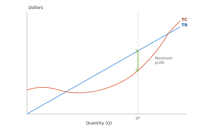
Figure 1: Profit Maximisation via TR and TC 

Moreover, the average fixed cost decreases as output increases. Thus, the average total cost can fall while the average variable cost is increasing. The relationship between both curves AVC and ATC, together with the Marginal Cost (MC) of production, is noticeable. At the same time, the marginal cost intersects with average variable cost and average total cost curves, creating a geometric relationship that helps manage two thresholds of decisions.

Shutdown Rule and Break-even Point

When price falls below the average variable cost, a firm loses more by operating than by shutting down, since it cannot even cover variable costs, let alone contribute to fixed costs. The situation is a shutdown rule. When the price level is between the average variable cost and average total cost, the company will produce at a loss in the short run. On the other hand, the price equal to the average total cost marks the break-even point of the production of the good. When production costs are below the average total cost curve, there is a possibility for the company to go out of the market and stop producing completely.

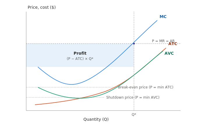
Figure 2: Cost Curves and the Shutdown/Break-Even Thresholds 

The diagram above lays out MC, ATC, and AVC together, with the profit-maximising quantity at the same Q* shown above. 

Short Run Versus Long Run

To understand the concept of the short run in contrast to the long run, we should consider the fact that fixed costs are a part of the costs in the short run while all costs are variable in the long run. It is important to remember that perfectly competitive industries tend to experience zero economic profit over time as firms leave any unprofitable market, a process that pushes the industry toward allocative efficiency. 

→ Read more about Short run and Long run

Real-World Example

Airlines provide a clear example of the shutdown rule because in some cases, airlines sell their seats at a price above fuel costs, as long as the price of the tickets is high enough.

At the same time, the shale oil industry in the US serves as evidence for the economic theory. When the price of oil fell, the companies with high fixed costs had to leave the market, while those with low AVC levels kept producing at the previous levels.

All theories show the application of the MC, ATC, and AVC as functions with the corresponding TR, MR, and AR business functions.